The Solar Model finds a big fall in TSI data that few seem to know about

Leif Svalgaard claims “TSI has not fallen since 2003”. It’s technically true in a sense, but demonstrably false when discussing 11 year smoothed trends (which is written on the graph he was criticizing). Willis Eschenbach sadly was carried along. This post is in response to an overheated thread at WUWT. Both men owe David Evans an apology.

The fuss is over the big fall in TSI. Leif Svalgaard said it was “almost fraudulent” that we claimed there was a fall in TSI since 2003 since there wasn’t a fall in this dataset. He says: “There is no such drop.” I say, look at the graph below, it’s even in your own data. Svalgaard provided the link to his TSI set, and we’ve included that line in the graph below. It’s the light-purple line. (Has he paid attention for the last ten years?)

In his rush to call it “totally wrong” and to declare “the model is already falsified” he didn’t notice we were talking about a trend in 11 year smoothed TSI, and the fall is evident in whole cycles (but takes some wisdom to find in daily or monthly data). I guess that’s a mistake that could happen to anyone — but some of us might ask politely before we started calling “fraud”, and saying things like “Mr Evans assertion is false [and I maintain seems to be agenda driven…” Likewise, Willis Eschenbach unskeptically follows: “as Leif points out, he’s using a bogus set of TSI data.” If skeptics toss out careless accusations, it rather cheapens the real ones.

Obviously the 11-year smoothed effect is news to Svalgaard, perhaps it’s news to a lot of people. It’s something David found because his Fourier work suggested a notch, and the Solar Model that was made with a notch filter predicted a big fall to come. From that David inferred there must have been a corresponding large drop in TSI and then he created the 11 year smoothed graph and found it (in response, it must be said, to an email from Lubos in April asking if there was an easier way to see there was going to be a big fall in temperature than through the model output).

The comments at WattsUp has been unseemly, and entirely unnecessary. (I’m sure it doesn’t help Anthony.) We will deal with other misunderstandings from the same thread (yes there were more) in a future post. The uninformed ad homs are a waste of time. What happened to common courtesy?

Compare the major datasets of TSI or proxies:

The major TSI datasets all agree there has been a large fall since 2003, in terms of 11 year smoothing (which is obviously required to remove the sunspot cycle and reveal the underlying trend). The SORCE/TIM reconstruction shows the fall starting in 1994. The “composite TSI” is that used by David to drive the model, averaging Lean 2000 (to the end of 2008), PMOD, and ACRIM (from the start of 1992).

As to whether the SORCE data should have been used in the Notch-Delay Solar Model — it’s rather trivially clear that since it starts in 2003 it’s not very useful for 11 year smoothed graphs, because there is only a single point of 11-year-smoothed data. It’s no use for finding the model parameters, because the delay of about 11 years means it cannot be used to check predicted temperatures against observed temperatures yet. And SORCE might be wonderful but it isn’t useful for Fourier analysis of long term climate cycles either (it’s hard to find an 11 year delay in only 11 years of data).

Strangely too, for a commenter who I hear is familiar with solar data, Svalgaard seems to forget that the last peak of solar cycles was 2001-2002, which is not visible in the graph he linked to (SORCE wasn’t operating then). Svalgaard compares data that starts after the peak with the next peak and says “they are the same” as if it means something. It’s a tad misleading (to be polite). I’m sure he didn’t mean it that way.

The graph below pretty clearly shows how TSI from the 2003 to 2012 fits — at least in the larger PMOD scheme of things (SORCE data only covers this short era). Yes, it’s technically accurate to say that TSI now is the same as 2003. Svalgaard declares ” If anything TSI is now higher than it were in 2003.” But it is obvious that the peak of the latest cycle is a lot less than previous ones.

In PMOD data (like SORCE data) obviously TSI now is similar to 2003. Equally obviously, that’s a meaningless comparison. The current peak is nothing like the last one.

Svalgaard thinks science is a bloodsport

Svalgaard emailed me this morning saying “science is a bloodsport”.

I replied that it “doesn’t have to be… You could use logic and reasoning instead.”

All the facts could be uncovered faster by honest enquiring minds without malice. People who brought preconceived assumptions about “motivations” and bad-will into a science debate failed to read what was put before them. We knew David’s work was going to be difficult, and that’s why we’ve released it bit by bit. They aren’t the only ones who have not read carefully enough.

Svalgaard admits reconstructions are “guesses”

Noteworthy is Svalgaard’s honesty about reconstructions. Commenter Brad, here asked why Leif used the term “TSI-guess” in his file label, Leif responded saying: “All so-called ‘reconstructions’ of TSI are Guesses. Most of them bad. The TSI-Guess.xls file is my guess.”

He elaborated:

TSI varies because the magnetic field of the Sun varies, and the field varies as the Sunspot Number does, so the variation of TSI is essentially that of the sunspot number [which is known] on top of a fixed background that does not vary. Based on the past decade of SORCE/TIM precise measurements of TSI, we can calibrate the sunspot number in terms of TSI. That gives me a Guess, which will not be correct in details, but will capture the gross features of the variation.

A brief history of TSI datasets

David Evans looked at all the major TSI datasets he could find in 2013, and downloaded the data available on 8 Aug 2013 when he froze the data used by the project. It’s harder to measure the sunlight than you might think, because there is a wide spectrum of light from UV to infra red. Everyone thought there was essentially no variation to measure up ’til late 1978 when people started observing it with satellites — it’s telling that TSI used to be called “the solar constant”. But there is really only one observed record that runs through the last 35 years, namely PMOD. ACRIM provides data from 1978, but before 1992 or so its results disagreed with PMOD and Lean (which is a reconstruction guided by PMOD). Like everything in climate, there is a war going over the adjustments and reconstructions and no one can agree. Fans of the IPCC now say the TSI was falling for decades, while others think TSI pretty much stayed high til the 23rd cycle and the 24th has been strikingly small.*

The PMOD dataset is the longest running continuous TSI record. ACRIM data got compromised by the Challenger Shuttle exploding, and then its results apparently didn’t quite make sense until the early 1990s. Bring on SOURCE, a new hot tool in 2003, which seems to work well. Lean and co used the PMOD data with sunspots during the same period and figured out a kind of calibration to use so we could estimate TSI from the old sunspot data. Yes, it’s difficult and we all wish Napoleon had fixed his satellite program, but it was not to be. The data is what it is. We are all doing the best we can.

Hmm. That’s a sudden adjustment in the reconstruction of TSI dataset?

The steep fall shown in the graphs for the predictions in part VIII is from 11 year smoothing of the PMOD and ACRIM data. And it’s still there in the updated data (see the update in post VIII). But a funny thing happened to the SORCE/TIM dataset. Anthony Watts covered the strange rearrangement of TSI reported on Feb 6 2014. The SORCE / TIM data changed rather a lot overnight. Previously there were four high peaks in the late 20th Century, but now there was only one, and it was the earliest.

Note the dramatic change in the last three peaks. (It’s a 3 second slow blink)

The animation makes it clear the shape of the last few peaks is quite different.

The next data battleground is going to be when the fall in TSI occurred. If it occurred in 2003 as per the PMOD and ACRIM data, then a corresponding fall in temperature is on the cards for about 2017. If it started in 1995 as per the new SORCE/TIM reconstruction now favored by the IPCC suggests, then the corresponding fall in temperature should have been evident from about 2006 — but since it didn’t happen that would mean the solar influence is weak. In the return of a previous theme, the measured data favors the former, while the later relies on reconstructions (the SORCE/TIM data only starts in 2003, and is not relevant to the 11 year smoothed values in the mid 1990s) that flatly disagree with the measured data.

The bottom line here is that perhaps SORCE/TIM is a better guesstimate of TSI than PMOD, but whatever PMOD is measuring seems to be a better predictor of Earth’s temperature. So in future if we can elucidate what makes PMOD useful and the new SORCE/TIM reconstruction not so much, then we may get clues as to the mystery force that operates with an 11 year lag. Obviously temperature is not following the SORCE/TIM reconstruction with an 11 year lag, but it does seem to follow PMOD.

———————————————————————————

Keep reading →

9.3 out of 10 based on 110 ratings

Are transfer functions meaningless (the “white noise” point)? Beware your assumptions!

Some people are claiming that the transfer function is meaningless because you could use white noise instead of temperature data and get the same notch. It’s true, you could. But the argument is itself a surprisingly banal fallacy. It looks seductive, but it’s like saying that it is meaningless to add 3 oranges to 3 oranges because you could add 3 oranges to 3 apples and you’d still get six!

It is trivially obvious that the transfer function will find a relationship between entirely unrelated time series, as any mathematical tool will when it’s misapplied. The question that matters — as with any mathematical tool — is has it been misapplied? What matters is whether the base assumption is valid, and whether the results will be a useful answer to the question you’ve asked. If the assumption is that apples and oranges are both pieces of fruit, and the question you ask is “how many pieces of fruit do we have”, then it is useful to add apples and oranges. But if you are trying to compare changes in fruit consumption, adding the two is mindless. So let’s look at the assumptions and the question being asked.

Assumptions first

Two assumptions were made before computing the transfer function. And before anyone complains that the whole project was a circular tautology — pay attention — the assumptions are temporary. They are a “what if” used to see if we get a meaningful answer. Later the assumptions are dropped and tested.

Assuming that:

1. Recent global warming was associated almost entirely with TSI.

2. The climate system is linear and invariant

…then, the transfer function from TSI to temperature is of great interest and sinusoidal analysis is appropriate.

David Evans has been explicit about both right from the start, but not all commenters seem to realize the implications.

The transfer function between TSI and Earth’s (surface) temperature will be meaningless if there is no causal link between TSI and Earth’s temperature. (Some people may need to read that twice).

This “link” could be an indirect one. It doesn’t mean that TSI itself is causing the change in temperature. It could, for example, mean that TSI is a leading indicator of other solar events that lag it by 11 years. It could be that those other events — say magnetic fields, solar wind, UV or other spectrum changes — are the ones actually causing the albedo changes that cause the temperature to change 11 years after the TSI changes.

By all means, if you have definitive evidence that changes in TSI cannot possibly be directly or indirectly associated with changes in Earth’s temperature, do let us know. It will save us a lot of time. Likewise, if you know of any reason why TSI can not possibly be a leading indicator for some other solar factor which acts with an 11 year cycle, please let us know. Some people are willing to declare they know that TSI cannot be associated with changes in Earth’s temperature. Some of us have an open mind. The solar dynamo is not completely worked out. Fair?

What about the question we are trying to answer?

As to the second part, what question was David Evans asking, and are the results useful? He made it explicit.

The initial aim of this project is to answer this question: If the recent global warming was associated almost entirely with solar radiation, and had no dependence on CO2, what solar model would account for it?

So is the discovery of a notch filter useful, and does it help to create a solar model? It certainly looks that way so far.

The model was constructed in the frequency domain. The main feature in the transfer function is the notch, so we tried building a similar notch in the model. The existence of the notch implies there has to be an accompanying delay (the timing seems unnaturally perfect, people are understandbly having trouble wrapping their heads around that). The delay was later found to likely be 11 years, which is not only the length of the major cycle of the solar dynamo but is borne out by other independent studies– such as Usoskin, Soon, Archibald, Friis-Christensen and Lassen, Solheim, Moffa-Sanchez, etc. (see post III). Later, a model based on an 11 year delay was found to produce reasonable results (see that hindcasting).

So the notch turned out to be very useful in building the model, giving two of the five elements in the model (the other three are the low pass filter, the RATS multiplier, and the immediate path for TSI, which were deduced by physical reasoning).

It would be better if there was a known mechanism. Of course, but Rome wasn’t built in a day, steady on. We are working on it. If people already knew what force X was then presumably they would have noticed its correlation with temperature and the climate problem would already have been solved, wouldn’t it? Some commenters, (those not focused on fallacies like argument from incredulity or the mechanics of publication time-tables) are being very helpful in gathering clues on force X — thank you!.

PS: The release?

And for those who are impatiently waiting the full working model, we’re working on it. There are a few last-minute things to sort out. The spreadsheet used data to August 2013 in the investigation, and was frozen months ago with that data. That’s the copy that is available to people who got advance notice. Now that we are releasing it, it would be nice to update the data, while preserving the original calculations. David is copying the Aug 2013 data and updating all the data. We are also figuring out the creative commons conditions that would be workable, and deciding how to manage suggestions, adaptations, and modifications. We suspect the normal open source software sites don’t deal with 20Mb Excel files which people can modify, but which are very difficult to track changes on (does anyone know of a similar project?). Right now the sciencespeak legal department, open science support team, human relations division and marketing arm are working flat tack. (That’s both of us. 😉 )

The biggest impediment at the moment is that some people still haven’t read the first posts we put up carefully enough. Even though we answered their questions personally in comments they still keep repeating the same points. Should we have kept the whole project secret until we had solved all these questions? Perhaps, but it’s been immensely helpful to get some feedback and help from some readers, and we didn’t know who would be the most useful beforehand. They have made themselves known.

On the other hand we’re being compared to Phil Jones and Michael Mann by one commenter, which we think is a tiny bit over-the-top, given that Jones and Mann are funded by the taxpayer and they spent years and used legal means to prevent their data being made public. To put a fine point on it, we got no income from taxes, and we owe the critics nothing. We also ask nothing of them (except, implicitly, patience and manners). Maybe that looks equivalent to a few people — we can’t see it. All the fuss, seriously, is flattering (if counter-productive).

Manners makes no difference to the scientific method, but ultimately the human practice of the Scientific Method is only ever advanced by … humans, and manners do matter. Science is never advanced by namecalling, misquoting, strawmen and personal attacks. Please quote us exactly, eh?

9.3 out of 10 based on 138 ratings

Weekend Unthreaded

I’m sure some people must be tired of discussing the solar model 😉

7.2 out of 10 based on 21 ratings

Sea level rise less than 1mm for last 125 years in Kattegatt, Europe — Nils-Axel Morner

Nils‐Axel Mörner has a new paper out (his 589th). For 60 years he has been tracking the coastlines close to him, and carefully isolated the exact part which appears to be the most stable. From that he shows that the real sea-level rise in Northern Europe is less than 1 millimeter a year since 1890. This is less that the 1.6mm trend in 182 NOAA tide gauges, and far below the estimates of the IPCC reports.

There is also no sign of acceleration in sea-levels for the last 50 years. (How much should Europeans spend to stop a 1mm annual rise that was already going in 1890 and has not changed much since then?) If anything, Nils work shows how difficult it is to measure true sea-level rise on land that shifts.

In this graph below, he compares the rise of most tide gauges with the Kattegatt region, and the IPCC results. This is only one result from one place, but it is based on thousands of readings from sites all around Kattegatt. His painstaking attention to extreme detail and empirical data stands in stark contrast to the IPCC where the trend depends heavily on adjustments. (Those adjustments appear to be based on a tide gauge in Hong Kong that is subsiding compared to the four other records nearby). Nils notes that people once thought true eustatic sea level changes would be the same all over the world, but this is not so. He remarks that the search for a meaningful mean global rate has become “illusive”.

Nils explained that the superb thing with the Kattegatt region is that we have both a perfect control on the crustal movements, as well as a number of fine tide gauges, so, we can separate the two factors in a way hardly possible anywhere else.

FIG. 1. SPECTRUM OF RATES OF SEA LEVEL CHANGES IN RELATION TO THE DISTRIBUTION OF RATE VALUES OF THE NOAA TIDE GAUGE STATIONS [18, 22, 24]. ESTIMATES OF RISE BY THE IPCC FOR YEAR 2100 (GREEN ARROWS) [1], SATELLITE ALTIMETRY (+3.2 mm/yr) [23], MEAN OF 182 NOAA TIDE GAUGE STATIONS (+1.6 mm/yr) [24], THE NEW DATA FROM THE KATTEGATT SEA HERE PRESENTED (+0.8‐0.9 mm/yr), AND THE VALUE FROM SOME KEY SITES (±0.0 mm/yr) [22, 24].

The rise since 1890 is consistent, slow, and linear.

FIG. 5. TIDE GAUGE RECORDS OF KORSÖR, NYBORG AND AARHUS AS PRESENTED BY NOAA [18]. KORSÖR LIES RIGHT AT THE ZERO ISOBASE OF UPLIFT, AND THE SEA LEVEL RECORD (+0.81 ±0.18 mm/yr) SHOULD HENCE REPRESENT REGIONAL EUSTASY. (His graph includes two other areas, not shown here) THIS IMPLIES THAT ALL THREE RECORDS GIVE A CONGRUENT RECORD OF A REGIONAL EUSTATIC RISE IN THE ORDER OF 0.8‐0.9 mm/yr (THE MEAN BEING +0.87 ±0.15 mm/yr). THIS TREND HAS REMAINED STABLE OVER THE LAST 125 YEARS.

To show how much work goes into analyzing land masses for their tilt and change in height, here is one graph of norther Europe. The boxed area (Kattegatt) lies on the edge in between areas which are moving in opposite directions.

Keep reading →

9.4 out of 10 based on 95 ratings

BIG NEWS VIII: New solar theory predicts imminent global cooling

To recap — using an optimal Fourier Transform, David Evans discovered a form of notch filter operating between changes in sunlight and temperatures on Earth. This means there must be a delay — probably around 11 years. This not only fitted with the length of the solar dynamo cycle, but also with previous independent work suggesting a lag of ten years or a correlation with the solar activity of the previous cycle. The synopsis then is that solar irradiance (TSI) is a leading indicator of some other effect coming from the Sun after a delay of 11 years or so.

The discovery of this delay is a major clue about the direction of our future climate. The flickers in sunlight run a whole sunspot cycle ahead of some other force from the sun. Knowing that solar irradiance dropped suddenly from 2003 onwards tells us the rough timing of the fall in temperature that’s coming (just add a solar cycle length). What it doesn’t tell us is the amplitude — the size of the fall. That’s where the model may (or may not) tell us what we want to know. That test is coming, and very soon. This is an unusual time in the last 100 years where the forecasts from the CO2 driven models and the solar model diverge sharply. Oh the timing!

Ponder how ambitious this simple model is — the complex GCM’s only aim to predict decadal trends, and have failed to even do that. Here is a smaller simpler model proffering up a prediction which is so much more specific. The Solar Model has not shown skill yet in predictions on such short time-scales, though it hindcasts reasonably well on the turning points and longer scales. It cannot predict ENSO events, and obviously not aerosols, nor volcanoes. But if the notch-delay theory is right, the big drop coming is larger than the short term noise.

As we head to the UNFCCC meeting in Paris 2015 where global bureaucracy beckons, a sharp cooling change appears to be developing and set to hit in the next five years. Yet consortia of five-star politicans are not preparing for climate change, only for global warming. Around the world a billion dollars a day is invested in renewable energy, largely with the hope of changing the weather. Given that 20% of the world does not even have access to electricity, history books may marvel at how screwed priorities were, and how bureaucratized science cost so much more than the price of the grants.

As Bob Carter has been saying for a long time, politicians need to prepare for everything the climate may throw at us — see Climate the Counter Consensus.

Global Cooling is Imminent

Dr David Evans, 27 June 2014, David Evans’ Notch-Delay Solar Theory and Model Home

If the Sun mainly controls the temperature on Earth, a turning point is almost upon us. (In the second part of this series of blog posts we will demonstrate that carbon dioxide is responsible for less than 25% of the global warming of the last six decades, so presumably the Sun is mainly responsible.)

1 Why It’s Going to Cool

The reason for the cooling is the dramatic fall in solar radiation that started around 2004. Here is a graph of solar radiation since 1610, when sunspots were first recorded. The brown line is the solar radiation, and it peaks every 11 years or so because of the sunspot cycle. We put an 11-year smoother through it to give us the red line, which shows the trends in solar radiation.

Figure 1: The recent fall in TSI is the steepest and one of the largest ever recorded (records go back to 1610).

UPDATE: This graph has been updated after the PMOD revisions to TSI in late 2013 or 2014. It makes very little difference. Compare the new graph to the original here.

There have been three big, steep falls in solar radiation in the last 400 years.

The first was in the 1600s. It led to the depths of the Little Ice Age, and the Maunder Minimum. This was the coldest period during the last 400 years. There used to be fairs on the ice in the Thames River in London, because it would freeze over for weeks at a time.

The second fall is around the time of Napoleon and it preceded the second coldest period in the last 400 years, called the Dalton Minimum.

The third fall occurred recently, starting in about 2004. This recent fall is as big as the fall in Napoleon’s time, almost as large as the fall in the 1600s, and it seems to be steeper than either of those falls. But the temperature hasn’t fallen … yet.

2 When

The timing for the cooling is indicated by the delay, which was deduced from the observed notch but has been independently corroborated to varying extents several times in the last decade (see Post III). The delay is most likely 11 years, though definitely between 10 and 20 years.

2004 + 11 = 2015.

Eleven years after 2004 is 2015, suggesting the cooling will start in 2015. However, 11 years is only the average delay, and the physical interpretation of the delay (see Post IV) suggests the delay is actually the length of the solar cycle—which has varied from 8 to 14 years, but averages 11 years. The current solar cycle is a long one, probably running around 13 years:

2004 + 13 = 2017.

So the cooling is most likely to begin in 2017.

The delay could be as much as 20 years, in which case the drop could be as late as 2024. Or it could occur as soon as 2014. An El Nino or La Nina could affect the timing too. At this stage, we don’t know. But by the end of 2018 seems fairly likely.

(Notice that so far we have only applied our physical understanding of the delay, and its implication of a powerful solar influence that is signaled by changes in solar radiation but acts after a period of time equal to the delay.)

3 How Much Cooling

How much cooling and how quickly? For that we turn to the notch-delay solar model, which hindcasts the last 240 years of temperatures reasonably well simply from the total solar irradiance (TSI). This model was developed earlier in this series of blog posts; see here for an overview and links.

The changes in solar radiation are tiny, and have an almost insignificant immediate effect on Earth’s temperatures. However the physical interpretation of the notch and delay (see Post IV) show that these little changes foretell the changes in a newly detected climate influence from the Sun, which we are calling “force X” for now. The effect on temperatures of changes in force X is 10 to 20 times as great as the immediate effect of changes in solar radiation (see Post VI). Force X works by modulating the albedo of the Earth, or the amount of solar radiation reflected straight back out to space without changing the heat of the planet, by clouds and ice and so on. Force X turns the tap that controls how much sunlight pours into the Earth’s climate system. This could be through UV, magnetic field effects, solar wind, or some form of electrical field.

Force X lags TSI by half of a full solar cycle of 22 years, which is to say, by 11 years on average. Therefore the changes in solar radiation over the last 11 years tell us what force X is going to do soon. It’s already baked in the cake; we can see a few years into the future.

Figure 2: Climate model driven only by solar radiation, with no warming due to carbon dioxide. See Post VII for explanation. Predictions shown by dotted lines. This instance of the notch-delay solar model used a constant delay of 10.7 years and shows cooling beginning in 2014.

UPDATE: The predictions have been updated with new TSI data from PMOD revisions in late 2013 or 2014. Again, there is little difference, compared to the original.

If the temperature on Earth is entirely controlled by solar effects, the cooling will return us to the temperature levels of the 1950s or even the 1920s, undoing the last 50 or 100 years of global warming in just a few short years.

The temperature data from land thermometers from 1850 to 1978 may have exaggerated past temperature rises. The solar model here trained on that data so it may be too sensitive, in which case the imminent cooling will not be as large as shown in absolute terms.

At least a small portion of the recent global warming was due to rising carbon dioxide, so the fall will not be as large as shown in Figure 2.

4 Solar versus Carbon Dioxide

Both the carbon dioxide and notch-delay solar theories agree with the warming observed during the 1900s, because carbon dioxide levels and solar radiation levels were both generally rising. So we cannot tell the models apart on recent performance.

However, over the next 10 years the theories strongly diverge. Carbon dioxide levels will continue to rise at much the same rate, so the carbon dioxide models predict warming over the next decade of about 0.2°C, plus up to 0.3°C of previously-committed warming not reflected in the temperature “pause” of the past 15⁺ years. Owing to the fall in solar radiation from around 2004, and making allowance for rising carbon dioxide, the notch-delay solar model predicts cooling of 0.2°C or more.

Figure 3: Comparing the CO₂and solar models. They show general agreement from 1900 to 2000, because carbon dioxide and solar radiation levels were generally rising, but they diverge sharply soon.

5 Theories and Falsifiability

Science is about testable hypotheses. Over the next decade, the changes in temperature will reveal which theory is more correct, the carbon dioxide model or the notch-delay solar model.

Here’s the criterion: A fall of at least 0.1°C (on a 1-year smoothed basis) in global average surface air temperature over the next decade.

If the criterion does not occur: Then the notch-delay solar model is falsified and it should be thrown away.

If the criterion does occur: Then carbon dioxide driven models are falsified, and they should be thrown away. (Note that the carbon dioxide theory predicts only warming over longer periods such as a decade, and we’ve already had a pause in warming for 15⁺ years.)

6 Old Temperatures

The Maunder Minimum from about 1645 to 1715 and the Dalton period from about 1790 to 1830 are generally reckoned to be the two coldest times in the last 400 years.

There was no global thermometer network before 1850, so for a global picture we have to rely on proxy data (ice-cores, pollen, marine sediments, lake sediments, tree-rings, etc.). The most comprehensive study is Christiansen and Ljungqvist’s huge proxy study in 2012, which used 91 proxies scattered around the world. We smoothed it by 25 years in Figure 1 because proxy data is uncertain and hazy.

Even the IPCC thought those two periods were the coldest in the last 400 years, before they went all hockeystick:

Figure 4: From the First Assessment Report of the IPCC, page 202.

Fig 5 (updated) IPCC Second Assessment Report, Fig 3.20 page 175, The SAR WGI first pdf). Decadal summer temperature index for the Northern Hemisphere, from Bradley and Jones (1993), up to 1970-1979. The record is based on the average of 16 proxy summer temperature records from North America, Europe and eastAsia. The smooth line was created using an apporximately 50-year Gaussian filter. Recent instrumental data for Northern Hemisphere summer temperature anomalies (over land and ocean) are also plotted (thick line). The instrumental record is probably biased high in the mid-19th century because of exposures differing from current techniques (eg Parker, 1994b)

UPDATE: We’ve replaced the graph originally posted (copied here) which was sourced via here. Thanks especially to William Connolley for the proof reading and to ThinkingScientist for accurately finding the actual SAR IPCC Graph above. It is entirely incidental to the Solar Model or its predictions, a mere side note here, not included in the main paper or the model, but we always appreciate feedback. The point remains that it has been long accepted that solar minima correspond to cooler temperatures on Earth. — Jo

7 What’s Next

This almost finishes the first part of this series of blog posts. The second part is about finding whether the carbon dioxide or solar model is dominant, from the evidence to date. This develops a method for computing the extent of causation, and finds that rising carbon dioxide levels were responsible for less than 25% of the global warming of the last 60 years.

The next post in this series is of the spreadsheet that contains all the data, code and the model behind the notch-delay solar theory. We have delayed releasing it so as not to preempt the blog posts, and to engender a more focused conversation.

The home page for the entire notch-delay solar theory is here. It includes links to all these blog posts, with summaries.

8.9 out of 10 based on 175 ratings

Color me skeptical – the Gore and Palmer paradox

The Fairfax press say the improbable Gore-Palmer play was a win for alarmists. The Australian calls it for skeptics and says Gore is a fool. I’m not calling anything until I see the fine print. Palmer says he’s met P.M. Abbott and he was ‘encouraged’ by his climate plan.

The only thing I can say for sure is that the science of CO2 is irrelevant to both Gore and Palmer. Everything else is a paradox. We’re not being told everything.

It seems now that Palmer’s amendments to repealing the carbon tax do not include an Emissions Trading Scheme (even the Fairfax press agrees). That makes it look like a skeptic win, but keeping the $10b Clean Energy Finance Corporation is a win for Gore, and so is keeping the RET (Renewable Energy Target) and the Climate Change Authority — it’s another government funded advertising unit for the carbon scare campaign. The more patrons who are dependent on the carbon-subsidies, the more pro-carbon lobbyists there are. And they lobby like their livelihood depends on it — because they have nothing if the government policies don’t prop up their pretend free market.

Why would Gore have any interest in standing next to Clive-Palmer-the-coal-magnate as he axes Australia’s carbon tax? Some suggest Gore was paid for the event, but the man got $100m from Big-Qatari-Oil selling his TV Channel — even a few million to be there yesterday (and we don’t know he got anything) would not make it worth his while. I don’t think Gore was here for anything bar the big game. He wants a global trading scheme (which might be worth more than the global oil market — we’re talking a $2T annual turnover). The rest is little biccies. A million here, a million there, so what? And Gore sheds no tears over the death of the coalition’s Direct Action Plan, because it was never really about actually reducing carbon emissions, was it? It’s about keeping Green Gravy flowing and window dressing.

More inexplicable is what Palmer gains from standing next to Gore. Part of Palmer’s appeal at the last election was that he wouldn’t support “carbon action” of any kind. Palmer, surely, is not aiming to win semi-Green voters to his voter base? Clive risks burning off more voters than he gains. This is not about the environment, and it’s not about voters, so what is it about?

Gore’s motivations seem easier to understand than Palmer’s. The election of Tony Abbott on a blood oath to get rid of the carbon tax is a devastating break in the global PR story about the so-called rise of “carbon trading”. It popped the bubble — and it’s no accident Gore is here just before it goes to the new Senate. He wants to limit that damage and rescue the narrative that a global carbon scheme is inevitable. It’s all about momentum, or rather the semblance of such. Gore wants to go to Paris in 2015 being able to say “Australia wants carbon trading”. Perhaps he can finangle weak agreements from all the countries named, which each nation thinks is never going to happen, then present them as a fait accompli at the UNFCCC and embarrass them into meeting their agreements?

The latest developments are that Senator Nick Xenophon is leaning on two of Palmer’s senators — Ricky Muir and Jackie Lambie — to support the Coalition’s Direct Action plan. A political consultant of Muir says he hasn’t decided. Lambie says “no way” to Xenophon’s suggestion.

9.4 out of 10 based on 71 ratings

Unbelieveable – Palmer to axe the tax, but vote for Carbon trading scheme?

This is not what PUP voters thought they were voting for… but the Big-Bankers will be happy.

Really? Clive Palmer holds the balance of p0wer in the new Australian Senate, due to start on July 1. He’s the coal magnate who made it clear he would get rid of the carbon tax. Now he’s palling up with Al Gore, and saying he’ll vote the tax down but only if we add a clause for an emissions trading scheme that is conditional on China, the US, the EU, Japan and Korea joining in too. Is this a meaningless dead-duck promise that is unlikely to happen, or is this the long softening up for the UN convention in Paris next year, when weak schemes (like China’s, where lots of permits are free) are used as leverage to call in the sub-clauses? I don’t think Gore would be flying out here if there was no chance this legislation would matter. At the very least he will use it to lean on other countries, as evidence that “Australia wants in”. At the very least this is about keeping the illusion of momentum going.

What is going on behind the scenes for this extraordinary turn-around? The man said only two months ago that he thought global warming was natural and 97% of carbon emissions came from nature. Clive the-coal-miner suddenly cares about carbon?

His long-awaited declaration on climate policy clears the way for Mr Abbott’s signature carbon tax abolition, but throws into doubt other aspects of the Coalition’s climate policies.

In a blow to the Abbott government, Mr Palmer said his Palmer United Party would use its decisive four votes in the Senate to block the proposed abolition of the money-making CEFC and would also move to legislate an emissions trading scheme with a starting price of zero dollars. — Sydney Morning Herald.

Keep the CEFC? The Clean Energy Finance Corporation

There would be enough support for the government to abolish the 20 per cent Renewable Energy Target, despite figures showing consumers would be better off if the target was kept, but the CEFC, which has turned a $200 million profit on investing in renewable energy projects, is likely to be retained on current numbers.

— also, Sydney Morning Herald.

Financial institutions benefit from trading schemes, but they don’t benefit from taxes (and they certainly don’t want “Direct Action”).

From Andrew Bolt h/t TonyfromOz and Bobl

Keep reading →

8.5 out of 10 based on 64 ratings

BIG NEWS Part VII — Hindcasting with the Solar Model

All models are wrong, some are useful. That’s how all modelers speak (except perhaps some climate scientists).

The barriers to making a good climate model are many. The data is short, noisy, adjusted, and many factors are simultaneously at work, some not well described yet. Climate modeling is in its infancy, yet billions of dollars rests on the assumption that CO2 will cause catastrophic warming and the evidence that most recent warming was due to CO2 comes entirely out of models. It’s important to focus on the pea:

“No climate model that has used natural forcing only has reproduced the observed global mean warming trend” (IPCC 2007)

It is a crucial plank that modelers say “we can’t explain the current warming without CO2”. Current climate models assume that changes in solar radiation have a small immediate effect and solar magnetic fields have no significant effect on Earth’s temperature. They do not consider the possibility that a solar effect may occur with an 11 year delay (equivalent to one solar cycle), despite the independent studies that suggest this. These GCM models cannot use CO2 to predict modern temperatures without amplifying feedbacks, for which evidence is sparse or even contradictory. They don’t predict the pause, or the upper tropospheric temperatures, or the Medieval Warm Period.

The total climate model described below can reproduce graphs based on a CO2 model, such as one used by GISS, but it can also produce graphs using the solar model developed in these posts, or a mix of both CO2 and solar. (This is the point where the solar assumption is dropped and tested.) The point here is simply to see if there is a viable alternative model to the CO2 model. It appears there is, which is not to say it’s finished, or can’t be improved, or cannot be presented better, or tweaked. At this stage it’s crude, but it exists.

There are 23 well funded ambitious global climate models that have been developed by international teams over the last 30 years, and a huge effort has been made by PR teams to make those models look good. The model below is one person’s work over 18 months with the aim of asking only, “is this possible” and “what can we learn?” The results are displayed with bare honesty and many caveats about how much (or how little) can be read out of them.

No model, much less one whose predictions have not been tested, is proof of any hypothesis. But they are sometimes good tools to tell us where to look. The notch-delay solar model is a viable alternative to the current CO2 models. It matches most major turning points of temperature (something CO2 models have struggled to do), and is used here back to 1770 — 100 years earlier than most. There’s a definite weak period with the 1950-1980 era where the atmospheric bomb test line resolves to have an improbably large effect. You might think the idea that nuclear tests cooled the planet in the 60’s and 70s is ridiculous. I certainly did. It’s something fans of CO2-theories have used to explain the cooling that Co2 based models can’t explain. Does it have legs? Hard to say, and worthy of a post on its own. But before you write it off, see John Daly’s site which has an interesting discussion page that compares bombs to Pinatubo eruptions, and points out atomic bomb testing went on in the atmosphere, despite the 1963 test ban treaty, until 1980 (thanks to the Chinese and French). Nuclear bombs contribute aerosol dust, but moreso, it’s radioactive too (a bit of a cosmic ray effect?). You might think it will rain out quickly, but bombs of 1Megaton reach up to the stratosphere above the clouds that rain. All up, 504 atmospheric nuclear explosions occurred between 1945 and 1980. A total of 440 MT were detonated (Fujii). It hangs around, C14 Radiocarbon levels in the atmosphere peaked in 1963 but the isotope stayed above natural levels for years – into the mid 1980s. (Edwards 2012). Fujii (2011) suggests atmospheric tests caused the “global stagnation“of that era and say it should be included in GCM’s. Maybe it isn’t as mad as it sounds?

The model has no aerosol component, which may or may not offset the cooling theoretically attributed to atmospheric bombs, nor does it have the Pacific Decadal Oscillation or Lunar cycles. The anomaly may be resolved if the model is expanded, or maybe it just means the delayed force from the sun is not the major driver — as we’ll explain in the next post, we’ll probably all have a good idea in a few years.

Solar TSI appears to be a leading indicator for some other (probably solar) effect, that we are calling “force X” for now. If that factor, quantified by TSI, was fed into current climate models, then those models would work with less forcing from CO2. Perhaps they would have produced better long term graphs, as well as fitting the recent pause and not requiring such a pronounced tropospheric hotspot. It might solve a lot of problems at once. Presumably projections of catastrophe would be subdued.

Lastly, compounding the many hindcast inaccuracies is the problem of inexplicable adjustments to temperatures (every skeptic will be wondering). It’s possible a model trained on raw temperatures curves (or older published datasets) may produce quite a different fit (which might be better or worse). For instance, if the land thermometer data from 1850 to 1978 exaggerates the general temperature rise then the solar model will be too sensitive — because it trained (or computed its parameters) on this data and “thinks” the TSI changes caused that amount of temperature change. Ultimately we won’t know for a few years whether it is right. (Bring on those independent audits please!)

The theory of the “delay” will be tested soon. It is falsifiable. We’re putting it out there for discussion. We have issued no press release, we aren’t selling a product (we’ll give it all away soon), nor do we demand your tax money. Judge it accordingly.

The bottom line is that modern climate models do not include any delayed force from the Sun. Saying that models don’t work without CO2, and no natural factors can explain the modern warming, is and always was, a fallacy known as argument from ignorance. — Jo

Hindcasting

Dr David Evans, 24 June 2014, David Evans’ Notch-Delay Solar Theory and Model Home

In the previous posts we built the notch-delay solar model. Now we are going to test it.

The solar model is given the TSI record from 1749 (the start of monthly sunspot records), and it computes the corresponding temperature in each month from 1770 from just the TSI data for the current and previous months. Then we compare this “hindcast” with the measured temperatures. We also test the CO₂ model to compare how it performs, and we test a mix of the CO₂ and solar models to show that they play together well.

Finally, we look at the significance (or not) of the solar model so far.

1 Our total climate model

The total climate model* includes the notch-delay solar model, a standard CO₂ model (two-compartments, with transient and equilibrium responses, computing temperature changes from the observed CO2 levels), a CFCs model (based on Lu 2013), and an atmospheric nuclear bomb tests model (based on the megatons exploded in the atmosphere, from UN reports). It can also apply all the forcings from the GISS model E, a mainstream climate model that released its forcings publicly in 2011—notably volcanoes, black carbon, snow albedo, and land use.

All these models can be switched on or off in any pattern within our total climate model. The total climate model has an optimizer to fit the model’s temperature output to measured temperatures, thus finding a set of optimal parameters.

We use composite TSI and temperature records for the measured TSI and temperature, as in the previous post. The composite temperature was put together from the main temperature datasets, instrumental back to 1880 then increasingly reliant on proxies, mainly the huge proxy study by Christiansen and Ljungqvist in 2012. Similarly the composite TSI record was constructed out of the main TSI datasets, using measured data where possible.

2 What if CO2 was the main driver?

To show how our “total climate model” works, let’s first fit a CO₂ model to the observed temperatures, assuming there is no delayed link between TSI and temperatures (that is, the mainstream assumption).

Let’s run the CO2 model with solar input as per the GISS model (that is, the immediate, direct effect of changes in TSI), with the volcanoes, black carbon, snow albedo and land use also from GISS, and the CFCs. The CO2 model was fitted to the measured temperatures and found to have an equilibrium climate sensitivity (ECS) of 3.4°C, agreeing with the IPCC’s central estimate of 3.3°C. The carbon dioxide theory fits the measured temperatures since 1800 fairly well in a very smoothed sense:

Figure 1: Total climate model without the solar model. It includes immediate warming due to changes in TSI as per the mainstream “GISS Model E” climate model. Thus, most of the warming must come from carbon dioxide. The estimated equilibrium climate sensitivity is 3.4°C, close to the central estimate of 3.3°C by the IPCC

The CO2 model produces a smooth increase in temperature, echoing the smoothly increasing CO2 concentration. Carbon dioxide by itself cannot begin to explain the jiggles in temperature on time scales from one to 10 years, so the carbon dioxide theory calls these jiggles “natural variability”—essentially meaning the bits they cannot explain.

3 What if solar effects were the main driver?

Now let’s run the notch-delay solar model, without any contribution from CO₂ or CFCs. In other words, we are running the solar model under the solar assumption, that the recent global warming was associated almost entirely with solar radiation and had no dependence on CO2. As explained at the start of these posts, we set out to build a solar model that could account for the recent global warming under that assumption.

So, we are now testing the proposition that the recent global warming could have been mainly associated with TSI rather than CO2.

There is monthly TSI data from 1749, when the SIDC monthly sunspot records start—they are a decent proxy for TSI, and along with Lean’s yearly reconstruction of TSI from sunspots are the only components of the composite TSI from 1749 to 1882. The step response of the notch-delay solar model takes about 15+ years to fully respond, so the model takes 20 years or so to spin up, and we begin the simulation in 1770. (During the Maunder minimum, from about 1660 to 1705, there were almost no sunspots, so the solar model has no way of estimating force X. Thus it cannot really be expected to work before about 1720 at about the earliest.)

Each monthly temperature computed by the solar model is computed only from the TSI data for previous months and the current month. This is the only data input to the solar model. We then add temperature changes due to volcanoes and so on from the other models, to form the temperature record computed by the total climate model.

The solar model computes the temperature for a given month by adding together all the step responses of the TSI steps of the previous months (that is, by convolution). The change in TSI from one month to the next is a “step” in TSI, and the temperature response to that step is as shown in the step response of the solar model in Figure 4 of Post VI, appropriately scaled by the size of the monthly TSI step. Yes this method is a little slow and there are faster methods, but this way makes it clear that we are using the step response and previous TSI data only—and anyway computers are faster these days, and the data series here have only a few thousand points.

We previously found the parameters of the solar model by fitting the model’s computed temperatures to the observed temperatures (and simultaneously fitting the model’s transfer function to the empirical transfer function). Therefore, so long as the temperature record computed by the solar model basically has the right shape, then of course it is going to fit the measured temperatures reasonably well. The question of how well it does is mainly going to depend on whether the model predicts the right shape of temperature curve, such as getting the turning points about right, because the fitting is going to ensure that the computed temperatures match the measured temperatures in a general sense.

The notch-delay solar model fits the measured temperatures reasonably well:

Figure 2a: 1770 – 2013 Total climate model when driven only by solar radiation, with no warming due to carbon dioxide. The solar model output is not explicitly shown here because having three lines close together (solar model, climate model, and observed temperatures) is too confusing, but it can be inferred by subtracting the other constituent models from the total climate model.

Figure 2b: 1900 – 2013: As for fig 2a, but for the last century.

The major temperature trends are all reconstructed, with major turning points about right, and the sizes of the reconstructed changes are roughly as observed. Therefore the notch-delay solar model could provide an entirely solar explanation for recent global warming, without any significant warming due to rising CO₂ or CFC levels.

The solar model reproduces a lot of jiggles, but gets the timing of them wrong as often as not, especially further back in time. This might simply be due to the fairly uncertain nature of the TSI data, which is reconstructed from sunspot numbers. Sunspot numbers themselves are uncertain because standards of what counted as a sunspot have varied over the years. And, as indicated by the physical interpretation of the delay in Post IV, the delay presumably is not constant but instead it is probably the length of the prevailing sunspot cycle, which averages 11 years but varies from 8 to 14 years. The solar model here is using a constant delay of 11 years. It doesn’t take much timing error to put an up-jiggle where there should be a down-jiggle. So there is some hope that, with better solar radiation data in future from satellites and a more complicated model with variable delay (the subject of future research perhaps, if there is sufficient interest), the solar model could explain some portion of “natural variability”.

Over the period of better TSI data from 1610, the TSI was clearly at a maximum from about 1950 to 2000. However the temperature kept increasing during this period, even though TSI plateaued. The delay in the solar model is 11 years, which pushes back that plateau from 1960 to 2010, but that is not enough to explain why the total climate model reconstructs rising temperatures throughout this period when it is based on the solar model and omits the CO₂ and CFC models. Here the output of the solar model is explicitly shown:

Figure 3: The solar model from 1900 as in Figure 2, but with the solar model output explicitly shown (in pink). From the 1950s through the 1990s (but mainly the 1960s), the solar model alone computes temperatures significantly warmer than actually occurred. In the total climate model this is counteracted by global cooling due to the atmospheric nuclear bomb tests, which put fine reflective dust into the atmosphere and apparently caused a mini-nuclear winter.

The answer found by curve fitting the total climate model to the observed temperatures is that global cooling caused by the atmospheric nuclear bomb tests may have counteracted the warming associated with the stronger TSI. This initially came as a great surprise to us, because the nuclear data had only been added as a bit of a joke and for completeness, but after a bit of research it started to look kind of plausible. The tests, conducted from 1945 to 1980 but mainly before 1963, put up fine dust that stayed high up in the atmosphere for years, reflecting sunlight back into space and lowering the incoming radiation [Fujii, 2011], and also dropping down radioactive nuclei that might seed clouds. Because the nuclear dust is in the stratosphere, there is no rain to wash it out. The required cooling from the tests is about 0.5°C at its peak in 1963, the year that the USA and the USSR agreed to discontinue atmospheric testing. (If the solar model is too sensitive because the warming of the land thermometer records is exaggerated, then less cooling is required.)

While this is only an answer found by numerically piecing together the test yield data with the output of the solar model and the observed temperatures, it fits. Maybe the nuclear winter hypothesis is partly correct. We feel it is likely to overestimate the effect.

Alternative causes for a cooling influence during the 1950s to 1990s could be pollutant aerosols and/or whatever caused global dimming, or even the Pacific Decadal Oscillation (PDO). With no data that quantifies their effects, the total climate model only had the nuclear bomb yield data to work with, but it is remarkable that the piece that fits the puzzle quite well is the atmospheric nuclear bomb test data.

4 Mix of CO2 and solar

There are now two solutions to the climate question:

If we assume global warming is mainly due to CO2 then we get the CO2 theory, and it fits the measured temperatures from 1800 (though not before).
If we assume that global warming is mainly associated with changes in TSI then we get the notch-delay solar model, which also fits the measured temperatures from 1800.

Obviously both assumptions cannot be true, but it may be that the true solution is a mix of both models—such as 40% of one model and 60% of the other. If both solutions fit the measured temperatures on their own, then any linear mix will also fit the data. Here is an example:

Figure 4: Total climate model when driven by a mix of solar radiation and carbon dioxide. The temperature changes computed by the solar model were multiplied by the solar factor of 70%, then the CO2 and other models were fitted. This mix was arbitrarily selected for illustration; do not read any significance into it.

This illustrates that the CO2 and solar models play together nicely. Assuming the climate system is linear for the small perturbations of the last few hundred years, the two solutions can operate almost independently and their temperature changes add (that is, they superpose).

If the optimizer is given both the CO2 and solar models to work with, it finds a solution that is mainly the CO2 solution and only a little of the solar solution. However this is only because the jiggles in the solar solution are wrong as often as not (Figure 2), which the optimizer finds worse than simply ignoring the jiggles and getting them right on average (Figure 1). So there doesn’t appear to be any significance in this, and we will have to find other means of determining the true balance between the CO2 and solar solutions.

5 Significance of the solar model

We have developed a solar model that accounts for the recent global warming, if that warming was almost entirely associated with solar radiation and had no dependence on carbon dioxide.

This is a viable solution to global warming, because:

It’s quantifiable, with a model that approximately hindcasts the observed temperatures. It is not just a concept with handwaving, or a rough one-off computation.
It’s got physical interpretations for all the parts. This is a physical model, not just curve fitting or an unexplained correlation.

In short, we have demonstrated that the global warming of the last two centuries could have been mainly associated with TSI rather than CO2. This overcomes one of the bedrock beliefs of anthropogenic global warming, namely that the recent global warming could not plausibly be due to anything other than CO2.

The most important element of the solar model is the delay, which is most likely 11 years (but definitely between 10 and 20 years). The delay was found here as a necessary consequence of the observed notch, but it has been independently corroborated to varying degrees several times over the last decade, apparently without its significance being noticed.

A major objection to substantial solar influence is the finding of Lockwood & Froehlich in 2007, who showed that four solar indicators including TSI peaked in about 1986 then declined slightly. However temperature continued rising for several years after 1986. This has been widely interpreted to mean the recent warming cannot have been due to the Sun. However, the delay can explain this: 1986 + 11 = 1997, about when global warming ended. Thus the delay overcomes another of the bedrock beliefs of anthropogenic global warming.

Conversely, without the delay, the objection of Lockwood and Froehlich appears solid and it is hard to see how a substantial solar influence is possible.

The weakest points of the notch-delay solar theory are:

The assumption of sufficient linearity of the climate system,
The need for the nuclear winter hypothesis to counteract the early part of the TSI plateau from 1950 to 2000, especially the 1960s.
The inability to precisely identify force X (see Post IV).

Some may challenge the discovery of the notch, but the notch implies a delay and the delay receives support from several independent findings.

What we have not shown so far in these posts is that the notch-delay solar model is true, or to what extent it is true. There is nothing in the posts so far to support the assumption that the recent global warming was almost entirely or even partly associated with solar radiation. On the material presented so far, the CO2 and solar solutions are both viable and no reasons have been given to suppose that either one is more influential.

The notch-delay theory provides a second, alternative solution to the climate problem, with a physical model and a plausible interpretation. No longer is climate a “one horse race”, where you are limited to either supporting the CO₂ theory or focusing on its deficiencies. We are now in a “two horse race” (though one horse is very new to the world and not fully introduced or fleshed out yet).

Regular readers of this blog are well aware that the CO2 solution has a lot of problems. Soon we will be turning to the second part of this series, where we will look at reasons for believing that the solar model is dominant and the CO2 solution is only a small part of the overall solution.

In the next post on this topic, we will use the notch-delay solar model for forecasting. This is where it gets interesting.

Notch-delay solar project home page, including links to all the articles on this blog, with summaries.

* Our climate model is in a spreadsheet that we will be releasing shortly. We chose to do all the work for this project, right from the beginning, in a single Microsoft Excel spreadsheet for pc. It’s not the fanciest or the fastest, but an Excel spreadsheet is the most ubiquitous and one of the friendlier programming environments. It runs on most computers (any pc with Excel 2007 or later, maybe on Macs with Excel 2011 or later), can hold all the data, makes nice graphs, and all in a single file. The models use VBA code, a form of the basic programming language that is part of Microsoft Office. The spreadsheet is professionally presented, and you press buttons on the sheets to make models run and so on. You can inspect and run or step through the code; it will be all totally open. Thank you for your patience, but giving away the spreadsheet early would preempt the blog posts and disrupt a focused discussion.

References

IPCC, Assessment Report 4, 2007, Working Group 1 Understanding and Attributing Climate Change, Chapter 9. Executive Summary. [IPCC site] Page 665

Edwards (2012) Entangled histories: Climate science and nuclear weapons research, The Bulletin of Atomic Scientists,

Fujii, Y. (2011). The role of atmospheric nuclear explosions on the stagnation of global warming in the mid 20th century. Journal of Atmospheric and Solar-Terrestrial Physics, Volume 73, Issues 5-6, April 2011, Pages 643-652. [PDF]

Lockwood, M., & Froehlich, C. (2007). Recent oppositely directed trends in solar climate forcings and the global mean surface air temperature. Proceedings of the Royal Society, 10.1098/rspa2007.1880.

Lockwood, M., & Froehlich, C. (2008). Different reconstructions of the total solar irradiance variation and dependence on response time scale. Proceedings of the Royal Society, 464, 1367-1385.

Lu, Q. (2013). Cosmic-Ray-Driven Reaction and Greenhouse Effect of Halogenated Molecules: Culprits for Atmospheric Ozone Depletion and Global Climate Change. International Journal of Modern Physics B, 27.

Pinker, R. T., Zhang, B., & Dutton, E. G. (2005). Do Satellites Detect Trends in Surface Solar Radiation? Science, Vol. 38, 6 May 2005, 850 – 854.

8.9 out of 10 based on 88 ratings

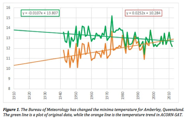
Don’t miss Jennifer Marohasy speaking in Sydney Wednesday

Jennifer Marohasy has been very involved in looking at Australian temperature data this year. She is speaking in Sydney on Wednesday about what she’s found. She’s talking about the new temperature dataset the BOM uses called ACORN, which they built after we asked them for an independent audit of their High Quality set.

Modelling Global Temperatures – What’s Wrong. Bourke & Amberley – as Case Studies

From Jennifer’s site: “The most extreme example that Ken found of data corruption was at Amberley, near Brisbane, Queensland, where a cooling minima trend was effectively reversed, Figure 1.” Jennifer has also raised her concerns (repeatedly) with Minister Greg Hunt.

Venue: The Gallipoli Club, 12 Loftus Street (between Bridge Street & Alfred Street), Sydney Time: 5.30 for 6pm

Additional Information: **Bookings from 11 June only ** BAR OPENS AT 5 PM – LIGHT REFRESHMENTS

Click here for info on how to book

8.9 out of 10 based on 71 ratings

Weekend Unthreaded

Sorry…we’ve been busy in the comments

8.5 out of 10 based on 29 ratings

Climate Rage: We absolutely cannot have… a rational conversation!

This post bumped to the top so it doesn’t get lost under the newer post: Solar Model Part IV below.

In The Rage of the Climate Central Planners, Jeffrey Tucker describes something we’ve all experienced. That moment where the social atmosphere turns suddenly poisonous. Climate Rage!

Namecalling is a tool to stop debate. It works to keep the wandering minds in the square. But the flipside is that sooner or later the smallest crack, the tiniest doubt, elicts a bizarre over-the-top response and the mismatch reveals the game. How many passionate skeptics are created in the moment a fence-sitter realizes that those who say they love the environment will risk friendships and burn relationships in order NOT to discuss it? For surely there is only one possible interpretation of Climate Rage.

“They really can’t allow a debate, because they will certainly and absolutely and rightly lose.”

“When that is certain, the only way forward is to rage.”

Keep reading →

9 out of 10 based on 219 ratings

BIG NEWS part VI: Building a new solar climate model with the notch filter

Open Science live — The story so far: Dr David Evans is building the O-D notch-delay solar model. It’s a much simpler big-picture approach than Global Climate Coupled Models. They use an ambitious bottom-up system where the models add up every small aspect in every small cell of the Earth’s climate atmosphere and oceans and try to predict everything, but the trap is the errors — small errors in 10,000 calculations add up to big-mush. David’s approach is top-down. He looks at the whole system from the outside, and doesn’t try to understand or predict each individual part. It’s a way of starting at the start — to shed light on the big forces and processes that happen as energy arrives on Earth, gets reflected, or blended, and eventually changes the surface temperature. His model won’t tell us what happens to rainfall in Sudan in 2050, but it might do what current models don’t and that is predict the global temperature.

The important development here is to complete the path of the energy flow in the most brutally simple way from Sun –> Earth –> Space. We know the sun provides heat through TSI or Total Solar Irradiance. But this is almost constant — it produces heat for sure, but possibly not much of the variation in temperature on Earth that we are interested in. The discovery of the notch filter means some other force (yet to be specified) from the sun acts with a delay of probably 11 years. This delayed force turns out to cause a lot of the variation in temperature. But Earth is not going to immediately warm or cool with every change. Energy collects in all kinds of pools and buckets before it ends up warming the atmosphere. So the effects of both incoming paths — immediate solar and delayed solar — get combined and run through a “low pass” filter — which blends and smooths the bumps.

Having discovered the pattern in the way TSI is tranformed into temperature, David builds the model with the filters to produce the same “transfer function” as he found in empirical data. Hopefully the model will mimic the overall processes without needing to know the details of all the parts. In a sense all models have to do this at some level. No climate model tracks each molecule or follows each photon. Will it work? It does a good job of hindcasting (and we’ll talk about that soon), but the real test will take a few years. Enjoy the quest to figure it out.

By the way, one of my favourite graphs is below — Figure 4 — some curves are intrinsically beautiful. — Jo

—————————————————–

Building a new solar climate model

Dr David Evans, 21 June 2014, David Evans’ Notch-Delay Solar Theory and Model Home

This is the last of the three posts in which we build the solar model. We assembled a notch filter, a delay filter, and a low pass filter in cascade in part III, in part IV we took a diversion to physically interpret the notch and the delay, and in part V we added the RATS multiplierto model the atmosphere on the yearly timescales of the TSI datasets.

In this post we assemble these four elements in their correct order, and add the immediate path for the TSI changes that obviously warm the Earth directly. This will complete the model. We finish by examining the step response of the model.

The Order of the Filters

The notch-delay solar model so far is simply a computational path from TSI to (surface) temperature that contains a notch filter, a delay filter, a low pass filter, and the RATS multiplier (which is a trivial “filter” whose transfer function is a constant). There are no other filters we can discern from the empirical transfer function, or from elementary physical theory. So with no more to add, let’s put these four in order.

The transfer functions of these four filters, when multiplied together, form the empirical transfer function. The transfer function of two filters in cascade is the products of their two transfer functions, so these four filters must be in cascade (that is, the output of one is the input of the next). But multiplication is commutative, so the empirical transfer function does not indicate their order. For that we turn to physical reasoning.

The filter whose place is most obvious is the low pass filter. It models the Earth as a bucket of heat with unreflected TSI pouring in the top, and its output is the radiating temperature. We can now place the other filters around it.

In the flow of computation the RATS multiplier goes immediately after the low pass filter, because its input is the radiating temperature and its output is the surface temperature. We then have the computational path covered from the unreflected TSI all the way to the output of the entire model.

The notch and delay filters intrinsically go together and are inseparable, and it does not matter if they go notch-delay or delay-notch. The only place left for them to go is between the input to the entire model, namely the TSI, and the input to the low pass filter, which is the unreflected TSI.

Therefore the notch and delay filters are modulating the albedo of the Earth.

Figure 1: The notch and delay filters modulate the Earth’s albedo.

The Immediate Path

The development to date only shows the delayed path from TSI to surface temperature. But obviously any changes in TSI also cause direct and immediate changes in the unreflected TSI, by changing the incoming heat from the Sun, so there is also an immediate path from TSI to the input of the low pass filter. This immediate path must therefore be in parallel with the notch-delay path from TSI to unreflected TSI.

The Notch-Delay Solar Model

Putting it all together, here is the notch-delay solar model. If the recent global warming was associated almost entirely with solar radiation, and if it had no dependence on carbon dioxide, this is how it would work:

Figure 2: Schematic of the notch-delay solar model.

Note the parallel paths:

The immediate path is for TSI, and has no effect on albedo. This is the direct warming effect of extra TSI.
The delayed path is for force X, which is the same as TSI but delayed and notched. Force X affects the albedo.

The parameters for the model were found by fitting the model to the observed temperatures since 1610, when yearly TSI data became available, though focused mainly on the last 100 and 200 years. Composite TSI and composite temperature records were created out of the TSI and temperature records analyzed earlier. In forming the composites, the offset of each dataset was adjusted so that the average values for overlapping datasets are the same, datasets were faded in and out of a composite gradually rather than entering the average abruptly, and instrumental data was preferred over proxy data. The fitting process found the model parameters such that the model best reproduced the composite temperature from the composite TSI and best produced a transfer function like the empirical transfer function found earlier.

The most important parameter is the delay parameter, which was found to most likely be 11 years but definitely between 10 and 20 years. The break period of the low pass filter was found to most likely be 5 years, though the possible range is from 4 to 25 years because it might be hiding over to the low frequency side of the notch. (It is very unlikely to be more than about the five years that other researchers have found, but the fitting process held open the possibility.) The most likely set of parameters is called the “P25” set of parameters. The values in P25 were rounded off to form the “P0” set of parameters, which has been used to illustrate the transfer functions and step responses of the filters during this development.

Keep reading →

9.1 out of 10 based on 71 ratings

Lubos and a few misconceptions

In typical style skeptics love to criticize, it is our strength. Sadly, diplomacy, manners, courtesy — burned at the door on a moment’s notice. Sigh. After five years in this debate you’d think I’d know not to expect respect or goodwill from every fellow skeptic. Call me naive, I don’t expect them to agree with me, just to be polite. If someone asks you for a review before they publish, would you congratulate them privately, ask questions, ignore the answers, ignore large parts of the paper, then later post those misunderstood points, without so much as a courtesy check first? Yes, I’m baffled too.

Hey Lubos, no hard feelings, but next time let us save you from posting unnecessary innuendo, irrelevant criticisms, and not-so-informed commentary. It only takes an email.

I groan. In a highly gregarious species, where power is clawed through high-order political games, schmoozing and collaboration, some skeptics still wonder why people who are bad with numbers but good with people, control the institutions, the publications and big budgets. The mystery of it all!

Anyhow, because it is out there (or was, I’ve reproduced it here)* and is being discussed, obviously we need to correct the errors. Lubos says he spent hours reading the paper but he doesn’t seem to be aware of several of the major points (hey, it’s a very long paper). Unfortunately, because Lubos thought we were suggesting something we weren’t, he concludes it’s all unlikely and bases quite a bit of his reasoning on this misconception. Here’s Lubos saying largely what we’ve said, but he thinks he’s explaining something new:

“Natural mechanisms on Earth just won’t produce a response function that happens to vanish exactly for the 11-year periodicity!”

We explained in this public post, the big paper, the FAQ, the small summary, and David wrote in personal email answers to him (April 11th), that we don’t think the delay and notching occurs on Earth. It doesn’t seem at all likely that the actual solar rays would take 8 minutes to arrive on Earth, then wait 11 years to warm the planet. The 11 year delayed effect is very odd – dare I say “mysterious?” (Perhaps I better not, lest it’s seen as “demagogy”, eh?)

Obviously the place to look for the notch and delay is on the Sun, where internal dynamics could easily produce an 11 year cycle, so easily, it already has. I don’t think Lubos realizes we are suggesting that the 11 year delay may have something to do with the timing of the 11 year solar magnetic flips? Perhaps it’s a coincidence the notching happens at the same time the sun’s magnetic field collapses and it flips its north and south pole. Perhaps it isn’t. Surely it’s an idea worth raising?

Again, I am ready to believe that the Sun has a significant impact on the Earth’s climate. But it must be either something else than the TSI, or the effect must be such that all the wiggles shorter than 20 years or so must be universally suppressed.

The argument that it is “due” to TSI, and “it’s not a mechanism on Earth” are both strawman: “it must be something else than TSI” he says — well yes, exactly. We go out of our way to say TSI is “associated with” with temperature, but does not “cause” temperature.

As for the “wiggles”, the evidence shows that all the wiggles shorter than 20 years are not equally suppressed. That is the point. Lubos is mixing up a low pass filter with the notch. The data most definitely does not suggest a low pass filter with a 20 year break point. (If it did, the lines in the graph Lubos reposted twice would be flat lines to 20 years, then bend down with a 45 degree decline to zero from there in the shorter frequencies.) The low pass filter appears weakly with about a 5 year break point. The low pass filter is a non-controversial idea — I don’t think many people would suggest that the Earth doesn’t smooth out the sun’s effects over at least a few years.

How about some manners?

For the sake of helping the skeptic world polish up on it’s key weakness, it’s time to discuss the forgotten topic of manners and communication. They matter in science. The truth may come out eventually anyway, but bad communication makes it slower, and bad manners risks burning off the independent valuable pool of volunteers who are providing a foil for the monopolistic bureaucratic influences of science. Strategically, it’s a win for skeptics to hold the torch on other skeptics, but a failure for them to waste time doing it on inaccurate and irrelevant points.

After five years of doing my genuine damnedest to improve science and advance human knowledge one tiny sliver at a time, I’m accustomed to being accused of blind faith or shallow marketing, but not from people who I thought shared the same goals.

Hence yes, lines like these (based on zero evidence) are disappointing. False motivations? Imputed intentions? Baseless accusations? We can do better.

There are climate skeptics who will endorse any claim or idea that goes against the “consensus”.

Obviously this does not apply (sometime I disagree with skeptics, sometimes I agree with the IPCC). Why say it?

David’s goal is to claim that the whole evolution of the global mean temperature – or a big portion of it, to say the least – and especially the 20th century global warming and its various intense episodes may be due to the Sun.

David’s goal is to learn more about what drives the climate, not to make false claims. Twice he dropped this project because the data didn’t seem to support the theory that there was a low pass filter (he went looking for the low pass filter, but eventually realized there was a notch obscuring it and the notch was the big deal). It’s what a scientist does. Let’s rise above the cheap shots. We don’t need pop psychoanalysis based on bad guesses.

I think that many of you will agree that the marketing point used as the title on Jo’s blog

For the first time – a mysterious notch filter found in the climate

is pure demagogy.

So when is it accurate science communication, and when is it “marketing” for an undescribed purpose? No one knew what might drive the notch, (or even that a notch existed) so mysterious seems pretty accurate, likewise, no one has described it before — looks like a first.

C’mon Lubos. Haven’t the footsoldiers in this David and Goliath battle at least earned the right to basic respect (and the right of reply) instead of half-baked, clumsy character slurs? Are they people and researchers or just dumb bloggers…

————————————-

Correcting Lubos’ Errors

Dr David Evans, 19 June 2014, David Evans’ Notch-Delay Solar Theory and Model Home

Here we correct several errors of fact or misleading impressions about the notch-delay theory made by Lubos.

1. Changes in TSI Did Not Cause the Recent Global Warming

Lubos says “David’s goal is to claim that” … “a big portion of” the “evolution of the global mean temperature”, “especially the 20th century global warming”, may be “due to” TSI. This is incorrect.

We have explicitly stated what our aim is, and that the recent global warming is NOT principally “due to” TSI. To repeat:

Part II: “The initial aim of this project is to answer this question: If the recent global warming was associated almost entirely with solar radiation, and had no dependence on CO2, what solar model would account for it?”
Part III: “We are building the solar model that would account for the recent global warming if it was associated almost entirely with solar radiation (notice that we didn’t say “caused”)”.
Part IV: We introduce the force deduced in the datasets, force X, as the main influence behind the recent global warming: “Force X has ten to twenty times more influence on temperatures on Earth than changes in the direct heating effect of TSI.” “While the effects on temperature of the tiny changes in the immediate heating effects of TSI are too small to explain the recent global warming, those tiny changes are a leading indicator of force X.”

2. Transfer functions are always output divided by input, in the frequency domain

After needlessly introducing complications such as convolution and integrals, and performing some handwavy and essentially correct math, Lubos says, as if he had uncovered something: “This frequency-based Evans response function is simply the ratio of the Fourier-transformed global mean temperature and the Fourier-transformed solar output!” (By “response function” he means “transfer function”.)

That definition of a transfer function is not only standard, it is explicitly stated from first principles in the Part II: “A transfer function tells how a sinusoid in the input is transferred through the system to the output. We are only concerned with amplitudes (that is, not phases), so its value at a given frequency is simply the output amplitude at that frequency divided by the input amplitude at that frequency. Dividing the orange line in Figure 4 by the orange line in Figure 2, we arrive at the empirical transfer function shown in Figure 5.”

3. There is no peak at 11 years in the temperature spectrum (i.e. there is a notch)

Lubos writes “What the near-vanishing of R~(f) for 1/f close to 11 years really means is that … the 11-year cycle isn’t present in the temperature data.”

Just caught on Lubos? The main point in the first substantive post is that the temperature record does not contain detectable temperature peaks at 11 years, which would corresponding to the peaks of TSI every 11 years. This is unexpected, and is the discovery. Under the heading “Spot the big clue. There is no peak at 11 years!” we said “The TSI peaks every 11 years or so, yet there is no detected corresponding peak in the temperature, even using our new low noise optimal Fourier transform!”

4. The notch is the starting clue

Lubos says about the absence of an 11 year peak in the temperature datasets: “This is a problem – potentially a huge problem – for any theory that tries to present the solar output as the primary driver even at the decadal scale and faster scales. … It makes the solar theory of the climate much less likely, not more likely. Suggesting otherwise is a case of demagogy.”

Not at all. It is the vital clue that leads us to the delay (which is corroborated at least in part by several studies), and then to the conclusion that an indirect solar force that is not TSI is potentially responsible for most of the recent global warming. This is unfolding in the blog posts already posted, and was available to Lubos in the main paper.

5. Notching originates on the Sun, caused by the synchronicity between two solar forces

Joanne has mentioned that Lubos is attacking a strawman with his arguments about “natural mechanisms on Earth”. This is a major point. We said as much so in the post on interpreting the notch and delay: “As far as we know there is nothing on Earth with a memory spanning multiple years. But there is one climate actor with an 11 year clock—the Sun.” We then proposed force X, which like TSI originates in the Sun, and showed the peaks in TSI every 11 years (on average) always exactly coincide with troughs in force X, which we propose as the notching mechanism.

Curiously, in one of his emails to me Lubos asked about exactly these “unnatural” mechanisms on Earth: “Concerning the unnaturalness, are you religious – what I really mean, do you believe in Intelligent Design?” (10 April). I replied (11 April) “No, I don’t believe in Intelligent design, but in logic, data, and reading carefully 🙂 … The 11 year timing (or more likely, the solar cycle length) almost certainly originates in the sun, presumably as two signals given off by different parts of the sun and 180 degrees out of phase. See Fig. 31. Force X lags TSI by 180 degrees of the 22-year Hale cycle, presumably. Hence the timing and the notching.”

6. The predictions are due to the delay

Prediction due to ringing? No, force X lags TSI by 11 years, so knowing what the TSI did we can predict what force X will do several years in advance—not Fourier analysis, just physical principles. From the post on the physical interpretation of the notch and delay: “Because TSI indicates what force X will do in about 11 years, the TSI record is also a record of future force X.”

Conclusion

It was the world’s sloppiest reading job. I asked for feedback when I first emailed it to him (“I’d really appreciate some feedback, especially if you disagree with or are uncomfortable with some aspects.”). But instead of sorting this out by email, he goes silent then writes a careless blog post that misrepresents the model. Unhelpful.

—————–

*Lubos took the post down. I told him that was unnecessary, I asked him to repost it. I’m reposting it here.

PS: Sadly Lubos has not coped well with this post. He refuses to correct his obvious mistakes, or quote me directly. My emails to him were polite and logical (read them in full here). I’ve asked him for an apology. Credit to him for publishing my comment on his blog. I remain baffled otherwise.

8.6 out of 10 based on 99 ratings

BIG NEWS Part V: Escaping heat. The Three pipes theory and the RATS multiplier

David Evans has analyzed the black box system that is effectively “Sunlight In, Temperature Out”, and found a notch, a delay, and a low pass filter. The problem then is to work out their order and to fill in any other bits needed by the model. This post then, doesn’t have big blockbuster moments (sorry), but these points need to be said.

Energy leaves Earth through a range of electromagnetic frequencies, but the bulk of them can be grouped into three main “pipes”. Radiation either comes directly off the land, oceans, ice and what-not on the ground, or it leaves via the atmosphere. Up in the air, carbon dioxide and water molecules do most of the work sending emissions of infra red to outer space. In the atmosphere, the radiating “surface” is a virtual concept and is effectively at different heights for different greenhouse gases. This is all non-controversial stuff, but a little difficult to see in your head. The three pipes are from the ground, from CO2 and from H2O.

There are three main “pipes” for heat to escape from Earth. A “pipe” is a group of electromagnetic frequencies which are radiated directly to space from the same emissions layer.

The next problem is that people have measured surface temperature (which is fair enough), and this is what the solar model is aiming to model. But it’s not the same temperature as the temperature of the complex “surface” that is radiating to space. The two layers are tied together in a sense. If the ground surface warms, the radiating surface will warm but not by quite as much. That means any model needs to understand the relationship between changes in the temperature of the radiating layers and the temperature on the ground (and on the seven seas). I’m sorry for anyone looking for a dog-fight here, but the multiplier in the Solar Model is boringly almost the same as the standard one used by mainstream climate scientists. We call it the RATS multiplier (Radiative Amplification To Surface) and its value is about 2.

Basically if it warms by 1 degree on the surface the RATS multiplier tells us it has warmed by about 0.5 degrees on the radiating “surface”. There were times when we thought it would be different, but it did indeed end up being about the same as the mainstream estimates. This is non-controversial stuff, but it’s important, and we’ll be referring back to the RATS multiplier and more importantly to the Three Pipes. – Jo

——————————————————————–

Modeling the Atmosphere

Dr David Evans, 18 June 2014, David Evans’ Notch-Delay Solar Theory and Model Home

This post is the second of the three posts in which we build the solar model. We already assembled a notch filter, a delay filter, and a low pass filter in cascade in part III, and in part IV we took a diversion to physically interpret the notch and the delay.

The output of the low pass filter is the record of changes in the effective temperature at which the Earth radiates to space, the “radiating temperature”. We then consider how the model will compute the changes in surface temperature from the changes in radiating temperature. It turns out to require just a very simple model of the atmosphere.

Three Pipes

The output of the low pass filter is the temperature of the surface of the Earth that radiates directly to space. This “radiating surface” is a virtual surface, consisting of different physical surfaces at different electromagnetic frequencies of radiation.

At the electromagnetic frequencies that are absorbed and emitted by carbon dioxide, the surface of the Earth is at the “one optical depth” of the carbon dioxide, where an observer from space is looking through sufficient carbon dioxide that they cannot “see” below that layer, on average. The carbon dioxide emissions layer is about 8 km up in the atmosphere at the tropics. It is effectively where all emissions from Earth direct to space at the carbon dioxide frequencies occur, because, on average, emissions below this layer are absorbed by the carbon dioxide (space cannot see those emitting carbon dioxide molecules, so they cannot see space).

The electromagnetic frequencies of the “atmospheric window” are those that pass through the atmosphere unimpeded. At these frequencies, emissions direct to space come from the surface of the Earth.

At the emissions and absorption frequencies of water vapor (which is the main greenhouse gas), the emissions layer is on average about 10 km up in the atmosphere at the tropics.

There are also other emissions layers for other greenhouse gases, but in this simple analysis we’ll ignore them because their effect is small.

Nearly all the heat lost by Earth goes through one of these three “pipes” to space, a “pipe” being a group of electromagnetic frequencies with the same emissions layer. The amount of energy flowing to space through each pipe increases with the temperature of its emission layer.

The “radiating temperature” of the Earth is the effective temperature of the radiating surface, and is simply the temperature as computed by the Stefan-Boltzmann equation for the emissions given off by the Earth. The temperature changes of the radiating surface are some sort of weighted average of the temperatures changes of the main three emissions layers.

Figure 1: The “radiating surface” is the virtual surface that radiates directly to space. It consists of different physical layers at different electromagnetic frequencies. The climate system is like a vessel containing heat, with three pipes through which heat can escape to space. Not to scale.

The RATS (Radiative Amplification To Surface) Multiplier

The low pass filter computes the changes in the radiating temperature, that is, the temperature changes that determine how much heat is radiated to space. But the output of the solar model is not this temperature, but the temperature at the surface. So how can the model compute the changes in surface temperature from the changes in radiating temperature?

Changes in the temperature of the radiating surface are basically transmitted down through the atmosphere to the surface. At the frequencies of the atmospheric window the radiating surface is also the surface of the Earth so no transmission is required, but at the carbon dioxide and water vapor frequencies the transmission is literally down through the atmosphere.

Keep reading →

8.7 out of 10 based on 85 ratings

When is your Green Charity too big? When it loses $5m currency trading

We need a Big News break for a day or so. Part V coming soon. Discussion is animated. — Jo

Financial speculation on currency sees Greenpeace lose €3.8m

[BlueandGreen] Campaign group Greenpeace lost €3.8m (£3m, or $5.5m AUD) after an employee took a gamble on the currency market in 2013, it has been revealed.

The employee responsible for losing the money took a gamble on the euro remaining weak against other currencies. However, the euro strengthened later in the year, resulting in the losses.

Greenpeace, save whales, trees, and help financial houses too. Who knew?

That $5m you were thinking of donating? Don’t bother, it wouldn’t have made any difference anyhow:

No Greenpeace campaign would suffer as a result of the loss, which would be absorbed by reducing expenses such as infrastructure over the next two to three years.

I don’t think this is quite the message Greenpeace meant to send.

Big-Green has truly become the Big-Business they pretend to oppose. Greenpeace has a total annual budget of around €300 million. It’s so big, it has to trade currencies, make property investments, and deal with “infrastructure”.

h/t Tim Blair See also the Sydney Morning Herald and The Guardian.

9.4 out of 10 based on 91 ratings

BIG NEWS part IV: A huge leap understanding the mysterious 11 year solar delay

Implacably, the discovery of a notch suggests a delay of anything from 10 to 20 years but most likely 11 years. (Don’t miss the delay post — two very big important concepts out in two posts). The big mystery is what could cause such a long delay in the correlation of solar radiation with temperatures on Earth?

David and I spent months wondering “what on Earth” could drive it. There were many possibilities though none of them seemed to be able to respond with the right timing: A resonant slop in ocean circulation could absorb extra energy, but it was difficult to see how the timing would be so tight with solar peaks. Likewise changes in ice or land cover. Then there are lunar cycles of 9 – 18 years, potentially generating atmospheric standing waves, but they were not synchronous with the sun.

Given that marine life can produce aerosol particles or carbonyl sulphide, we wondered if blue green algae or phytoplankton were the key. I particularly liked the idea that life on Earth would evolve to try to take advantage of the little extra energy arriving at regular intervals. But it’s unlikely, though not impossible, that microbiology would act after an 11 year delay. They could respond in weeks or months — but that type of response would not produce “a notch” in the transfer function. I spent most of 2013 spotting tantalizing 8 – 12 year cycles in papers on everything from arctic tundra to jet streams. All of which were interesting, but none of which would sit quietly for 10 years and then spring to life.

In the end, the answer was so prosaic, so beautiful — of course, the only possibility for a delay so perfectly timed with solar cycles was within the sun itself. Have we been fooled by a language slip? “Peak” solar activity doesn’t mean a “peak” in magnetic activity, actually it’s the other way around.

Think about the timing: At the peak of the sunspot cycle, while the sun is producing its maximum solar irradiation, it turns out that the Sun’s magnetic field is collapsing through its weakest moment. (Marvel at Figure 1 below.) The solar radiation only varies a little through the cycle, but the dynamo of the solar magnetic field is undergoing profound changes — flipping in polarity from North to South or back again. This causes the notch.

We don’t know exactly how this collapsing magnetic field reduces the effect of solar radiation on Earth. One obvious candidate is Svensmark’s cosmic ray hypothesis. He theorized that during the months of the weakest magnetic field the Earth loses its shield against cosmic rays, seeding clouds. But the mystery force might be electrical, or work through UV, or be something else entirely. Nonetheless, it was a leap to finally connect so many studies.

(This was a memorable “aha” moment — We did enjoy!.) — Jo

——————————————————-

Physical Interpretation of the Notch and Delay

Dr David Evans, 17 June 2014, David Evans’ Notch-Delay Solar Theory and Model Home

[Logically this post belongs a little later in the series, but some people seem so interested in the physical interpretation of the notch and the delay that we’ll jump forward in the story a little for a bit. So please excuse me for dragging a couple of things in from left field while I explain this, but I am under editor’s orders.]

The notch was observed in the data, and the delay was inferred from the notch. But what are the physical explanations for the notch and the delay?

The biggest clue lies in the delay, which we’ll take here to be the most likely value of about 11 years, though it could be as low as 10 years or as high as 20 years in the curve fitting.

The delay in the solar model says that today’s temperatures are more influenced by the level of solar radiation 11 years ago than by the level either 5 or 25 years ago. So something to do with climate has a memory of 11 years; the delay is not simply due to a dissipative element, like a store of heat in the ocean that declines at a certain rate.

(The heat store of the oceans is almost certainly the main element in the low pass filter, which is a dissipative element with a time constant, but that is quite separate from the delay. If a dissipative element dominated the response to TSI then today’s temperatures would be more influenced by the TSI of 5 years ago than of 11 years ago, but it’s the other way around.)

As far as we know there is nothing on Earth with a memory spanning multiple years. But there is one climate actor with an 11 year clock—the Sun.

The Sun’s sunspot cycle has an average length of 11 years, although it varies from 8 to 14 years. The Sun’s full cycle is actually 22 years long on average, consisting of two consecutive sunspot cycles, one with the Sun’s magnetic field in each orientation.

Also, the notching suggests that there is a countervailing force that counteracts the TSI peaks in the global surface temperature. This countervailing force would have to synchronized to the TSI peaks. While it might be a force that reacts to the onset of a TSI peak, a simpler explanation is that it originates on the Sun like the TSI and is thus synchronized to the TSI. *

We will soon deduce from the solar model that the notch and the delay work by affecting the albedo of the Earth (the fraction of solar radiation that is reflected straight back out to space by clouds, snow, ice etc. without warming the Earth, about 30%). We will also find by looking at the proportional changes in solar radiation and albedo that over the last few decades that the effect on temperature of albedo modulation has been at least six times greater than the immediate heating effect of variation in solar radiation. So it appears the notch and delay are associated with a powerful indirect solar influence that modulates the Earth’s albedo.

It is important not to prejudge what this influence is, so let us call this influence “force X” for now. Therefore the existence of “force X” is formally proposed:

If force X is larger, the Earth gets warmer.
Changes in force X lag behind changes in solar radiation by the delay, which is most likely half of the full solar cycle, or 180°—force X and TSI are in anti-cycle. The delay is the time between peaks in sunspots, which averages 11 years but varies from 8 to 14 years.
Force X affects the Earth’s temperature by changing its albedo.
Force X increases when the Sun’s magnetic field is stronger, and is weakest when the Sun’s magnetic field is reversing its polarity.

This last property is because peaks in solar radiation and sunspots coincide with reversals in the Sun’s magnetic field, as shown in Figure 1.

The Sun’s magnetic field reverses polarity every sunspot cycle, about every 11 years, and it occurs just as the TSI and the number of sunspots are peaking. In the reversal, the Sun’s north pole gets swapped with its south pole, so the magnitudes of some aspects of the solar magnetic field go briefly to zero, and presumably all aspects of the various solar magnetic fluxes are at a minimum. For example, the magnitude of the solar polar magnetic shown in Figure 1 field drops to zero before rebounding as the polar field reverses polarity.

This synchronicity of peaks in solar radiation with troughs in force X accounts for the observed notching. Just as the TSI peaks the warming from force X is at a minimum, so the peak in the direct warming effect of TSI is counteracted by the trough in warming from force X. Presumably the combined influence of the peak in TSI and the trough in force X is less than the precision of the temperature record.

(By the way, it was Joanne who noticed the synchronicity of TSI peaks with magnetic field reversals and made the connection to the notch and delay.)

Figure 1: When sunspot activity peaks, solar radiation is at a maximum but the solar magnetic field is at its weakest because it is reversing polarity. (This figure merely illustrates the timing; the solar polar field is but one aspect of the Sun’s magnetic field, and it is not proposed that this is force X.)

Although we can deduce its presence in the datasets, at this stage it is not known what force X is. We cannot measure some signal on an antenna pointed somewhere and say “that is force X”. Conversely, nearly every measured variable has been compared to temperature, so if someone was measuring force X they probably would have noticed by now.

The obvious candidate for force X is some aspect of the solar magnetic field that is responsible for deflecting cosmic rays so that they do not hit the Earth as often as they would otherwise. More cosmic rays hitting the Earth may create more microscopic cloud nuclei, which form more clouds, which reflect more solar radiation back into space, lowering the unreflected TSI entering the climate system and thus cooling the Earth’s surface. When the appropriate component of the solar magnetic field is stronger, it warms the Earth by protecting it from cooling cosmic rays. Thus, a solar magnetic field could modulate the albedo of Earth. When solar radiation peaks, force X is momentarily weak and the cosmic ray shields are down.

It is possible that force X is not related to cosmic rays. For instance force X might be electric and modulate the ozone in the Earth’s stratosphere, or otherwise affect the Earth’s atmosphere by some electrical connection. Solar magnetic fields are known to directly influence weather near the Earth’s poles, and may influence mid-latitudes via the global atmospheric electric circuit (Lam et al 2013). Or there may be solar influences which are not explainable yet (e.g. Sober 2010). Or it might be that solar UV modulates algae or plankton which in turn modulate albedo (Beckman, 2014). Yoshimura in 1996 found that the TSI leads some index of the solar magnetic field by 10.3 years, and posited that the Sun could affect the Earth’s climate “through two channels”.

Or it might be more than one of the above.

While the effects on temperature of the tiny changes in the immediate heating effects of TSI are too small to explain the recent global warming, those tiny changes are a leading indicator of force X. Tremors in the near-constant level of solar radiation foretell what force X will do in 11 years’ time. Because TSI indicates what force X will do in about 11 years, the TSI record is also a record of future force X.

Figure 2: Symbolic diagram of the Sun’s influence. The Sun influences Earthly temperature by two forces, solar radiation and force X, where changes in the former lead the latter by half a full solar (Hale) cycle. The influence of force X on changes in Earthly temperatures is about 10 to 20 times the influences of changes in the solar radiation.

Force X has ten to twenty times more influence on temperatures on Earth than changes in the direct heating effect of TSI (a result we will show later). TSI no doubt has vastly more energy than force X, but the changes in TSI are proportionally very small. Indeed, the level of TSI was thought to be constant until satellites were able to measure it more closely and found minor variations, and it used to be called “the solar constant”.

Force X affects the albedo of Earth, affecting how much solar radiation gets reflected straight back out to space. Force X is like a tap, a small force controlling the much larger flow of solar radiation into the Earth’s climate system.

Keep reading →

8.4 out of 10 based on 119 ratings

Unthreaded again

Look just because some people want to talk about something other than the new solar theory….

8.2 out of 10 based on 19 ratings

BIG NEWS Part III: The notch means a delay

UPDATE: July 21 Thanks to Bernie Hutchins, David found a problem with the code, which means the notch no longer guarantees a delay. The delay still likely exists (see the other evidence in the references below) but this post, particularly figure 2 needs correction and updating. – Jo

Strap yourself in. The Notch in the Earth’s response to incoming solar energy means that every 11 years (roughly) the solar energy peaks, and at the same time the climate’s response to the extra energy changes. What on Earth is going on?

The thing about notch filters that is hard for anyone who isn’t an electrical engineer to understand is that it appears to start working before “the event” it is filtering out. This is obvious in the step response graph. That’s Figure 2 – which shows what happens where there is a sudden step up in solar radiation (the brown line). The blue line shows the temperature response, which paradoxically starts to “rise” before the step up even occurs. This makes no sense, of course. Electronic engineers know that a [non-causal] notch filter always means a delay. Something triggers the filter before the event begins and the notch filter responds after a delay.

By mathematical inference David shows that there ~~must~~ be a delay. Later, by fitting the solar model to the measured temperatures, the delay is found to most likely be around 11 years (but is definitely between 10 and 20 years).

There is some empirical support for this from Lockwood and Froehlich’s paper, and also from Usokin, Archibald, Solheim, Soon, and Moffa-Sanchez.

The solar model also has a low pass filter, as well as the notch-delay combo. All the little flickering short rises and falls in solar radiation would not show up in Earth’s temperature. A low pass filter blends or smooths these short term cycles as the energy is absorbed by systems like the oceans. Only longer sustained changes in radiation make a difference, as heat either accumulates or dissipates over longer periods. The transfer function suggests (loosely) that changes lasting less than about 3 years make less and less impact on temperatures. — Jo

Building the Model Part 1: Deducing the Delay

Dr David Evans, 16 June 2014, David Evans’ Notch-Delay Solar Theory and Model Home

We are building the solar model that would account for the recent global warming if it was associated almost entirely with solar radiation (notice that we didn’t say “caused”), and had no dependence on carbon dioxide. Here we assemble the first three parts of the model, a notch filter, a delay filter, and a low pass filter.

1 The Notch

In the previous post on exploring the data, we found that the most prominent feature in the empirical transfer function was the notch, which filters out the 11-year “hum” from the Sun.

The notch is a very curious fact. Solar radiation warms the Earth, providing nearly all the heat as incoming radiation—visible light, UV, infrared, and so on. So we’d expect the extra radiation from the Sun every 11 years to produce corresponding peaks in temperature here on Earth. Yet it doesn’t.

We have chosen to investigate what happens if the recent global warming was associated almost entirely with changes in solar radiation and has no dependence on carbon dioxide — the “solar assumption”. Obviously the solar assumption cannot be entirely true, and it is later discarded in the development of the solar model. It is only needed for finding the approximate parameters for the model, and it does not ultimately impact on whether the model is appropriate or not. This parallels the original development of the carbon dioxide theory, which temporarily assumed that carbon dioxide caused almost all of the global warming since 1800 — the “carbon dioxide assumption” — in order that the parameters of the carbon dioxide model could be found by curve-fitting it to the measured temperatures.

Using the solar assumption we curve-fitted a notch model to the measured temperatures, to find the approximate size and shape of the natural notch filter. It is more instructive to show the notch filter we eventually found by curve fitting the entire solar model (which contains a notch filter) to the measured temperatures, because that way we can build up the model’s transfer function piece by piece so that it matches the empirical transfer function. (The two notch filters are basically similar except for a different overall amplitude multiplier, that is, a vertical shift in the transfer function diagram.)

Figure 1: The transfer function of the notch filter in the solar model. Uses the P0 set of parameter values for the solar model, which are the rounded off versions of the parameters later determined to best fit the observed temperatures.

Ok, it’s notch shaped, and the notch is at 11 years, as we’d expect. (We are only concerned with the amplitudes, because we cannot adequately detect the phases of the sinusoids in the climate datasets.)

But what is much more interesting becomes apparent when the notch filter is portrayed in the time domain, as the step response. The step response of a system is what the output does when the input instantaneously steps up by one unit.

Figure 2: The step response of the notch filter in the solar model, corresponding to the transfer function in Figure 1. It is non-causal, that is, the response starts before the stimulus!

Notice that the step response starts several years before the step-up, which violates causality — it is impossible. In our universe, a response can only come after the corresponding stimulus. The non-causality of the step response of the notch filter in Figure 2 is not a fluke: in any electronic notch filter without an accompanying delay, the step response is blatantly non-causal. Notch filters by themselves are intrinsically non-causal.

2 The Delay

How we know there is a delay

When engineers design a filter whose transfer response has the desired shape of amplitude, but which is non-causal and therefore impossible, they simply include a delay with the filter. Adding a delay does not change the amplitude of the transfer function of the filter, it only changes the phase of the transfer function. The delay shifts the entire amplitude part of the step response to the right in diagrams such as Figure 2, without changing its shape, as if the time axis were replaced with a new time axis.

For example, the step response of the combination of the notch filter in Figure 2 and a 7 year delay is the blue line in Figure 2 shifted 7 years to the right. Just imagine sliding the blue line 7 years to the right — the dagger of the notch would move from year 0 to year 7. (Notice this would almost but not quite make the response causal, because the response would almost be zero before the stimulus begins. A delay of about 8 or 9 years would be sufficient to make it causal and therefore possible.)

Keep reading →

8.8 out of 10 based on 60 ratings

BIG NEWS Part II: For the first time – a mysterious notch filter found in the climate

This is the first of many posts. It is primarily about the entirely new discovery of a notch filter, which electrical engineers will immediately recognize, but few others will know. Notch filters are used in electronics to filter out a hum or noise. You will have some at home, but everyone seems to have missed the largest notch filter running on the planet.

This post is also about the broad outline of the new solar model. It’s a O-D (zero-dimensional) model. Its strength lies in its simplicity — it’s a top down approach. That solves a lot of problems the larger ambitious GCMs create — they are a bottom up approach, and effectively drown in the noise and uncertainty. This model does not even attempt to predict regional or seasonal effects at this stage. First things first — we need to figure out the main drivers of the global climate.

Here David explains why sinusoids are such powerful tools. Some of the most important graphs here are in frequencies — that’s where we non-EE’s (Electrical Engineers) will have to concentrate. Pay attention to the logarithmic scale on the bottom. 1,000 year cycles are on the left, and 1 year cycles are on the right.

There is a lot to cover. As you read, good skeptics will be thinking of criticisms and questioning assumptions. That’s all excellent, please bear in mind we have asked many of these at length already (like, is it fair to assume linearity?) and this is a short introductory article. There is a lot to discuss. We assume, but only temporarily, that the Sun’s radiation might be associated with all the warming (note I didn’t say “cause”). This assumption is used for the investigation and then dropped and tested. It parallels what CO2 driven models do — they assumed CO2 caused all the warming. They just got stuck on the “testing” step. Also, David used Fourier analysis to investigate the datasets and find the filters, then used those filters he discovered to build a model. This two stage approach means skeptics may spot red flags that are relevant to one stage, but made irrelevant by the second stage. I’m flagging this at the start in the hope that we generate more constructive criticism.

No time? — skip to Figure 5 and 6 for the most important action! Look at the spike down at 11 years. See how it happens in all the datasets. (Figure 6 was the moment when Bob Carter sat up dead straight in his chair).

— Jo

——————————————————————————————————–

Discovering the Notch

Dr David Evans, 15 June 2014, David Evans’ Notch-Delay Solar Theory and Model Home

The carbon dioxide theory is clearly inadequate, as readers here know only all too well. So we wondered if the changes in the Sun might be causing some of the recent global warming. That is, the global warming over the last few decades, maybe back to 1800 or so.

Solar radiation and temperature

The best and most obvious solar datasets are those for total solar irradiance (TSI), or the total energy from the sun at all electromagnetic frequencies — mainly visible light, but also UV and some infrared. These datasets estimate the total energy from the Sun falling upon the plane that is at the average distance of the Earth from the Sun (1 AU, or astronomical unit). This TSI data is thus deseasonalized, so it cannot tell us anything about what is happening on time scales of less than a year or at frequencies greater than one cycle per year (this will become important later). TSI is measured in Watts per square meter (W/m²).

The temperature we are most interested in is the one for our immediate environment, the “global average surface air temperature”, namely air temperatures at or near the surface averaged across the entire planet. When we use “temperature” without qualification in these posts, we mean this temperature. “Global warming” is the rise in this temperature.

The initial aim of this project is to answer this question: If the recent global warming was associated almost entirely with solar radiation, and had no dependence on CO2, what solar model would account for it?

Let’s build that solar model

We are envisaging some sort of black box, whose input is TSI and whose output is temperature.

The climate system is approximately linear for small perturbations such as have occurred since the end of the last ice age. It is common in climate modeling to assume that the climate system is linear. The climate system is also “invariant”, which just means that its properties do not change significantly with time. So we assume that the climate system is linear and invariant, at least for the last few hundred years (and presumably as far back as the end of the last ice age).

The way to analyze a linear and invariant system is with sinusoids (aka sine waves). A sinusoid has a frequency, an amplitude, and a phase. Sinusoids are special for linear invariant systems, because:

If the input is a sinusoid, then the output is a sinusoid at the same frequency.
At each frequency, the ratio of output to input amplitudes and the difference between the output and input phases are always the same.
Behavior at one frequency is unaffected by what is occurring at other frequencies.

Lots of systems are linear and invariant, such as free space for electromagnetic fluctuations, which is why sinusoids and Fourier analysis are so ubiquitous in our analysis of the universe. While Fourier analysis can also be used for mere curve fitting, its true significance and power is that sinusoids are eigenfunctions of all linear invariant systems.

So let’s analyze the TSI and temperature datasets in the frequency domain. That is, we will recast them as sums of sinusoids.*

Keep reading →

9 out of 10 based on 142 ratings

Weekend Unthreaded

More action coming very soon, in the meantime, a space for all the things that are not the solar model…

(UPDATE: It’s posted!)

8.5 out of 10 based on 23 ratings

Recent Posts

Svalgaard thinks science is a bloodsport

Svalgaard admits reconstructions are “guesses”

A brief history of TSI datasets

Hmm. That’s a sudden adjustment in the reconstruction of TSI dataset?

Assumptions first

What about the question we are trying to answer?

Global Cooling is Imminent

1 Why It’s Going to Cool

2 When

3 How Much Cooling

4 Solar versus Carbon Dioxide

5 Theories and Falsifiability

6 Old Temperatures

7 What’s Next

Hindcasting

1 Our total climate model

2 What if CO2 was the main driver?

3 What if solar effects were the main driver?

4 Mix of CO2 and solar

5 Significance of the solar model

Building a new solar climate model

The Order of the Filters

The Immediate Path

The Notch-Delay Solar Model

How about some manners?

Correcting Lubos’ Errors

1. Changes in TSI Did Not Cause the Recent Global Warming

2. Transfer functions are always output divided by input, in the frequency domain

3. There is no peak at 11 years in the temperature spectrum (i.e. there is a notch)

4. The notch is the starting clue

5. Notching originates on the Sun, caused by the synchronicity between two solar forces

6. The predictions are due to the delay

Conclusion

—————–

Modeling the Atmosphere

Three Pipes

The RATS (Radiative Amplification To Surface) Multiplier

Financial speculation on currency sees Greenpeace lose €3.8m

Physical Interpretation of the Notch and Delay

Building the Model Part 1: Deducing the Delay

1 The Notch

2 The Delay

Discovering the Notch

Let’s build that solar model

JoNova

Find Things

Register for emails

Recent Comments

Statistics

Handbooks

Most commented

Archives

Tags

Links

Categories

Books